Two-Wheeled Self-Balancing Robot

2025 — 2026

Robotics coursework at Shanghai Jiao Tong University: an LQR controller and a simulation environment modelling an inverted pendulum under external forces, implemented and tested in MATLAB and Simulink.

MATLAB
Simulink
Control theory
Robotics

Designed an LQR controller for an inverted pendulum subject to external disturbances.
Built the simulation environment alongside it, so the controller was tested against the model rather than tuned by hand.

The problem

A two wheeled robot has no third point of contact, so standing upright is not a stable state. Left alone it falls, and the only thing it can do about that is drive its wheels. Staying up means continuously driving underneath its own centre of mass.

That makes it a textbook inverted pendulum, and the coursework was to design a controller that holds it steady while something is actively trying to push it over.

How it works

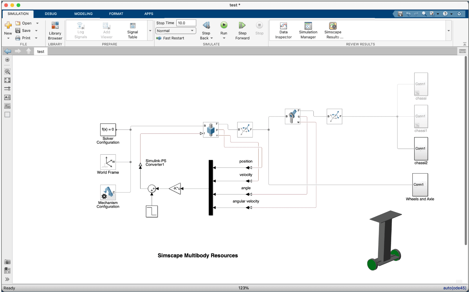
The Simscape Multibody model in Simulink. A solver configuration, world frame and mechanism configuration feed the plant on the left. The plant's position, velocity, angle and angular velocity are tapped off as signals, summed against a step reference and fed back through a gain block into the body, which connects to the chassis and the wheels and axle subsystems on the right. — The Simulink model: the multibody plant on the right, the state fed back through the gain block on the left.

The robot is modelled as an inverted pendulum on a cart, where the cart is the wheel axle. The state is the body's tilt and how fast it is tilting, together with the position and speed of the wheels.
Those equations are linearised around the upright position. Balancing only ever happens near vertical, so a linear model is accurate in exactly the region the controller operates in.
LQR chooses the feedback gains by minimising a cost that sums state error and control effort over time. Instead of tuning gains one at a time, you say in the Q and R weights how much a degree of tilt costs relative to motor effort and solve for the gains from that.
The controller drives the wheels from the full state, so a tilt is corrected by moving the base under the body rather than by fighting the lean in place.
The Simulink model injects external forces into the plant, so the controller is tested against being pushed rather than only against a starting tilt.
Controller and simulation were built together, which means a gain change could be replayed against the identical disturbance instead of against a slightly different one.

The model running

The animation below is the Simscape Multibody visualisation of the same model. The robot holds itself upright while the wheels drive back and forth underneath it, and the drift across the frame is the controller trading position for balance: it lets the base run rather than let the body fall.

The simulated robot, a flat body on two green wheels, holding itself upright while the wheels drive underneath it and it travels across the frame. — Simscape Multibody visualisation of the balancing run, sped up to fit five seconds.

What I learned

Q and R are where the design actually lives. Solving for the gains once the weights are set is mechanical. Deciding how expensive a degree of tilt should be compared to motor effort is a judgement about the robot you want, not about the algorithm.

Linearising is a promise about a small neighbourhood, and it is easy to forget that the model stops being honest once the robot leans far enough. A controller can look flawless in simulation and still have a lean angle past which nothing recovers it.

Building the simulation alongside the controller changed how the tuning went. Because a disturbance could be replayed exactly, each set of gains was comparable to the last one instead of being judged against a different push.