Natural Gas Price Forecasting

2026

A next-day price model for Henry Hub natural gas futures, built from price history, storage levels and weather. A gradient boosting model is measured against a SARIMA baseline, and both report a 90% prediction interval rather than a bare number, because a forecast you cannot put a range on is not one you can act on.

Python
LightGBM
SARIMA
Time series forecasting
Quantile regression
SHAP
pandas

Cut mean absolute error from $0.76 to $0.33 per MMBtu against the SARIMA baseline over a 49-day holdout, with prediction intervals roughly 3.7 times narrower.
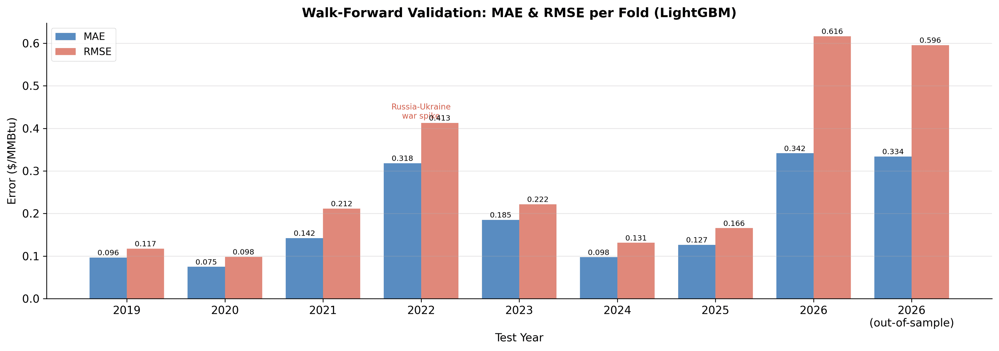
Validated with eight expanding-window walk-forward folds spanning the COVID demand crash, the Russia-Ukraine spike and the 2026 winter move.
Predicts the daily price change rather than the price level, so the model cannot score well by echoing yesterday.
Found our own sharper intervals under-cover at 79.6% against a 90% nominal, and reported that rather than widening them after the fact.

The problem

Natural gas is priced on weather that has not happened yet. A cold snap three weeks out moves the front-month contract today, and anyone buying gas for a plant or a portfolio has to commit before they know. So the useful question is not really what the price will be tomorrow. It is how wrong that guess could be.

Most forecasting coursework stops at a point estimate and a table of error metrics. We wanted the interval to be a first-class output instead, because that is the part a procurement or hedging decision actually consumes. A model that says $3.40 is not useful. A model that says $3.40 and is honest that the range is $2.90 to $4.10 is.

The target is the next-day close of the Henry Hub front-month contract, in dollars per MMBtu. Three sources feed it, all pulled live from APIs rather than shipped as a fixed extract: daily settlement prices from Yahoo Finance, weekly underground working gas storage from the US Energy Information Administration, and daily temperature from Open-Meteo, converted into heating degree days. That covers 2010 through March 2026, about 4,074 trading days.

How it works

Line chart of natural gas prices over the first ten weeks of 2026. The actual price sits near three dollars, runs up to seven dollars and forty-six cents in late January, then falls back within days. The LightGBM line follows the same shape a few days behind, while the SARIMA line stays flat near three dollars seventy throughout. — The 2026 holdout. LightGBM tracks the January spike a few days late; SARIMA flatlines through it.

Twenty-three features go into the model: price lags at 1, 3, 7, 14 and 30 days, rolling means and standard deviations, calendar seasonality, a linear trend index, one-day returns, storage level and its week-over-week change, heating and cooling season flags, heating degree days, and a volatility regime label.
The model predicts the daily change rather than the level, and the price is rebuilt afterwards by adding the predicted change to yesterday's close. Predicting the level directly gives a flattering error score for a model that has learned nothing except to repeat the last observation.
The baseline is SARIMA, with orders selected by auto_arima on AIC and then refit in SARIMAX so the intervals could be controlled. It sees only the price series, which is the point of it as a baseline.
The main model is LightGBM, 500 trees at depth 6. Three further models are trained at the 0.05, 0.50 and 0.95 quantiles using LightGBM's quantile objective, and those form the 90% band. Quantiles fitted independently can cross, so bounds that come back inverted are swapped and the median is clipped into the band.
Leakage is the thing that quietly ruins a time-series result, so it is blocked in four separate places. Every rolling window is shifted a day before it rolls. The weekly storage series is joined backward so only figures already released on that date are visible. Degree days are forward-filled and then lagged. Regime thresholds come from expanding quantiles over history rather than quantiles of the whole dataset, which would leak the future into the past.
Validation is walk-forward with an expanding window, always training from 2012 and testing one year forward. Ordinary k-fold cross-validation would train on 2024 to predict 2019, which is not a forecast.

Results

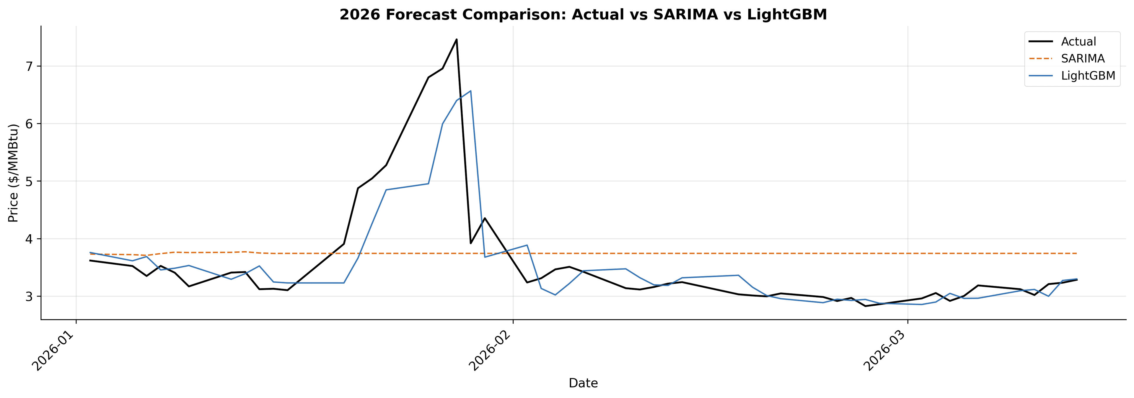
Over the 49 trading days from 2 January to 13 March 2026, held out entirely from training, LightGBM cut mean absolute error by 56% and mean absolute percentage error by 59% against the baseline, while producing intervals about 3.7 times narrower.

Grouped bar chart of mean absolute error and root mean squared error for each walk-forward test year from 2019 to 2026. Bars are low and flat from 2019 to 2021, rise sharply in 2022, settle again through 2024 and 2025, and rise again in 2026. — Error by test year. The two tall years are the 2022 war spike and the 2026 winter move.

SARIMA: MAE $0.76, RMSE $1.05, MAPE 19.75%, interval coverage 85.7%, average interval width $2.01.
LightGBM: MAE $0.33, RMSE $0.60, MAPE 8.04%, interval coverage 79.6%, average interval width $0.54.

What the error tells you

The single clearest result is in the holdout chart above. In late January 2026 the price ran from about $3.10 to $7.46 and collapsed back inside a fortnight. SARIMA predicted a flat $3.73 for the entire ten weeks. That is not a bug; it is what a univariate model does once you push it far enough past the last observation it saw, and it converges on the series mean. LightGBM caught the move about three days late, which is worse than useless for trading it and genuinely useful for knowing it is underway.

Across the walk-forward folds the error tracks how strange the year was. Calm years sit around $0.08 to $0.14 of mean absolute error. The 2022 fold, containing the Russia-Ukraine spike to $9.68, rises to $0.318, and the 2026 fold to $0.334. A model of a commodity market is really a model of its quiet periods, and the honest way to report it is per regime rather than as one pooled average.

What we learned

Sharpness and coverage trade against each other, and we ended up on the wrong side of it. Our 90% band held only 79.6% of actual values, which our own calibration rule flags as miscalibrated, while the far clumsier SARIMA band passed at 85.7% purely by being wide enough to be uninformative. The narrow interval fails exactly during the January spike, which is the one week anybody would have wanted it. A narrow interval that breaks under stress is a worse product than a wide one that holds, and the fix is conformal calibration rather than widening the band by hand until the number looks right.

SHAP puts one-day returns and the previous day's price well ahead of everything else, with storage and degree days landing second-tier. That is worth stating carefully. It says the model leans on momentum, not that momentum drives the gas market, and the two are easy to conflate when writing up a feature importance chart.

The obvious gaps are all in the inputs rather than the model. There are no macro variables at all, so oil prices, LNG export volumes and production are invisible to it. Nothing was hyperparameter tuned. Weather comes from a single coordinate at the geographic centre of the United States, standing in for the demand of an entire continent. Any of those would likely buy more accuracy than a better model architecture would.